


GLr01: "Brain decoding: toward real-time reconstruction of visual perception" -> Arxiv - 2310.19812
Breaking down - 'Brain Decoding: Toward Real-Time Reconstruction of Visual Perception- Arxiv - 2310.19812'—exploring MEG-based models, deep learning, and AI-driven neural representation learning.

Welcome to GLr01, the first entry in the GreyLattice Research (GLr) series!
First and foremost, thank you for being here. Your curiosity—no matter how small—plays a role in shaping the future of Neurotech. This series, [GLrx], is dedicated to breaking down complex research papers from first principles, making ground-breaking advancements in the field accessible to everyone.
Join me as we explore the latest innovations and unravel the frontiers of Neurotechnology.
Note:
This post is quite long and I understand if you would like to skip to certain sections or read certain parts of the blog alone. In that regard, Substack conveniently provides a sort of index that should appear on the left side while reading this blog(only on the site ) using which you, the reader, can skip to any section or subsection as you please.
I have also provided an index that used title links below for the app users.
Thank you for being here, let’s get back to the blog.
Index
(1) Author and Paper Information
(2) Introduction
(3) What Have They Achieved from This Research? / Key Findings
(4) Formulating the Problem Statement (Mathematically)
(4.1) Key Variables & What They Represent
(4.2) In Simple Terms
(5) Training Objectives
(5.1) Training Brain-Image Mapping with CLIP Loss (Retrieval Portion)
(5.1.1) What is CLIP?
(5.1.2) How CLIP Works
(5.1.3) Why Use CLIP Loss for Brain-Image Retrieval?
(5.2) Applying CLIP Loss to Brain-Image Mapping
(5.2.1) Why Do Both Directions Matter?
(5.2.2) Loss Formula
(5.2.3) Breaking It Down
(5.3) Training Brain-Image Mapping with MSE Loss (Generation Portion)
(5.3.1) Loss Formula
(5.3.2) Breaking It Down
(5.4) Final Loss Equation
(5.4.1) Breaking It Down
(5.5) Why Not Just Use MSE Loss?
(6) The Brain Module
(6.1) About the Model
(6.2) What is a Multi-Layer Perceptron?
(6.3) What Role Does It Play in Converting the Intermediate Output of Y(hat)agg from the Shape of F′ to F?
(6.4) Optimizing the Brain Module
(6.5) Postprocessing of MSE Outputs
(7) Image Module, Generation Module, and Optimizations on Latent Space
(7.1) Generation Module: From Latents to Images
(8) Time Windows — When Should Brain Activity Be Captured?
(9) Training and Computational Considerations
(10) Evaluation of the Model
(10.1) Retrieval Metrics (Matching MEG-Derived Latents to Correct Images)
(10.2) Generation Metrics (Assessing Image Reconstruction Quality)
(10.3) Real-Time and Averaged Metrics (Handling Multiple Image Presentations)
(11) Datasets Used and Pre-processing Performed
(11.1) Addressing Limitations in the Original Data Split
(11.2) Comparison with fMRI-Based Models
(12) The RESULTS
(12.1) Retrieval Performance: Which Latent Representations Worked Best?
(12.1.1) Key Findings
(12.1.2) Performance Comparison: Deep ConvNet vs. Linear Model
(12.2) Which Representations Were Most Effective?
(12.3) Understanding the Two Test Sets
(12.4) Why Do Some Representations Work Better?
(12.5) Deep Learning vs. Linear Models: A Clear Winner
(12.6) Final Takeaways
(12.7) Now, Coming Back to Generation
(12.8) Why Are Low-Level Details Missing? Comparing MEG and fMRI Reconstructions
(13) Wrap Up — There Was a Lot to Cover, But We Are Finally Done (Mostly…)
(13.1) Related Works
(13.2) Impact
(13.3) Limitations
(13.4) Ethical Implications
(13.5) Conclusion
(14) Sources
I came across this paper while looking for relevant research works for a personal project that I have been working on, and I found this work extremely insightful and fascinating.
Therefore, I decided to break it down and help my blog readers understand the insights I gained from trying to understand this research, and simultaneously start a subseries for my Blog called (GLr)(GreyLattice research). Let’s dive in!
(1) Author and paper information
This paper was authored by 3 amazing research scientists(Yohann Benchetrit, Hubert Banville and Jean-Rémi King) who work at Meta (and who I wish to work with on these amazing projects one day) with one of them(Jean) also being associated with Perceptual Systems Laboratory at ENS(École Normale Supérieure) university which is associated with the prestigious PSL university in Paris, France. This work was published on the Arxiv platform on 14th March 2024.
(2) Introduction
Let’s start with the abstract. What is the objective of this research? Why conduct this research?
When a person sees an apple on a table, multiple things happen, the major events being the light rays reflected off the apple and the table that are visible to the person’s eyes, hit the retina; These are then processed by the photoreceptor cells present in the eye that converts this light into electrical signals or neural signals which travel from the retina to the brain, this is the moment when the person “sees” the image.
The signals created throughout this process - of a person viewing an image, can be measured using a technique called fMRI(functional magnetic resonance imaging). Once recorded, these signals can be interpreted to understand how and why the brain works the way it does, and also how these signals are used to see what a person sees. Very cool, right?
But the current technique(fMRI) that is used to decode signals from the brain has a limited temporal resolution(≈0.5 Hz), meaning it can only capture brain activity at about one image per 2 seconds. This makes it unsuitable for real-time applications.
What does temporal resolution mean exactly? It’s defined as the amount of time needed to revisit and acquire data for the same location or how frequently a system can capture or record data over time. Now, considering that fMRI has a frequency of 0.5 Hz, it signifies that to capture a single measurement, it takes 1/0.5 = 2 seconds.
Therefore, the researchers propose an alternative method to read brain signals called magnetoencephalography (MEG), which is a neuroimaging technique that has a resolution of approximately 5000 Hz …. :o
This is significantly higher(10,000 times) than the fMRI technique and revolutionary in the study of brain waves and the functioning of the brain.
So, 5000 Hz essentially signifies that the amount of time taken for a single measurement is approximately (1/5000 = 0.0002th of a second). This level of measurement makes real-time research on brain waves possible, meaning researchers can now track brain responses for rapidly changing stimuli.
If at any point you questioned this → When does the brain create these signals for which these techniques are used to record and then eventually interpret the signals? That’s a good question!
Remember the electrical or neural signals created by photoreceptor cells reacting to light? These electrical signals from the retina are passed to the retinal ganglion cells, whose axons(the elongated thin middle part/ portion of the neuron cell that connects the cell body to the synapse(ending) in a neuron) form the optic nerve(the nerve is primarily responsible for sending these signals to the brain from your eyes as it is the nerve that directly connects a persons eyes and the brain). So these signals are now received by the optic nerve.
Now, the optic nerve carries signals to the lateral geniculate nucleus (LGN) in the thalamus, which processes visual information before sending it to the visual cortex.
What are all these complex terms?
Thalamus - Your thalamus is an egg-shaped structure in the middle of your brain. It acts as a relay centre for the brain for all sensory information except smelling(discrimination). So it takes the signals received from any and all sense organs and makes sure each of these signals is sent to the correct regions of the brain for processing. It filters signals to distinguish important from unimportant ones and so plays a major role in sleeping, focus, and wakefulness.
LGN(lateral geniculate nucleus) - The part of the thalamus that is assigned for vision tasks, relaying visual information and signals. The LGN sends these signals to the visual cortex.
Visual Cortex: A part or region within the Occipital Lobe( a region at the back of the brain where visual signals are processed). This region is where the brain interprets or processes what we see and is made up of different areas (V1, V2, V3, V4, IT - lol we have an IT department) each responsible for processing different aspects of an image from the signals gained:
V1 (Primary Visual Cortex) → The brain’s first "image processor"; detects basic features like edges, orientation, and contrast.
V2, V3, V4 → Add complexity, recognizing shapes, colours, and movement.
IT (Inferotemporal Cortex) → The final stage where the brain understands objects, faces, and scenes.
This layered processing turns raw retinal signals into meaningful images, objects, and concepts. So we essentially have a light-wave decoder.
So does the MEG record only these signals and make sense of what we see?
No, this is one of the main components of a set of signals that the MEG records for this research.
What are all the kinds of signals it records to be processed by the model?
MEG captures the electromagnetic activity of neurons, meaning it records:
Feedforward signals from the retina as they pass through the visual system. - THIS IS DESCRIBED ABOVE
Feedback signals where the brain modifies and reconstructs perception.
Internally generated signals (like imagination, memory-based vision, and predictive corrections).
(2) & (3) are new signals generated by the brain while interpreting and understanding signals from (1). For context:
As the information moves from V1 to higher areas (V2, V3, V4, IT, and prefrontal cortex), the brain starts generating its own internal signals:
Prediction signals: The brain predicts what it expects to see and fills in missing information.
Memory-based reconstruction: If an object is partially hidden, the brain fills in the gaps based on experience.
Attention signals: The brain decides which part of the image to focus on and amplifies relevant features.
This is called recurrent processing or feedback processing because the brain is not just passively receiving signals—it is actively modifying and interpreting them.
The above signals captured by the MEG help researchers decode not just what is seen but also how the brain processes and reconstructs images.
Note:
The difference between MEG and fMRI is based on the medium through which they measure brain activity:
fMRI Temporal Resolution (~0.5 Hz = 1 sample every 2 seconds)
MRI indirectly measures brain activity through blood flow changes (BOLD signal).
Since blood flow is slow, fMRI can only take one measurement every ~2 seconds (0.5 Hz).
If a person looks at multiple images rapidly, fMRI struggles to distinguish fast changes in brain activity because it takes too long between measurements.
MEG Temporal Resolution (~5000 Hz = 5000 samples per second)
MEG records electrical and magnetic signals directly from neurons, which change much faster than blood flow.
MEG captures 5000 measurements per second, allowing researchers to see moment-by-moment brain activity in real time.
Now that we have understood what these brain signals are, how they are generated, and what these neuroimaging techniques truly record, we move forward with the paper and its research methods.
To decode these brain signals and reconstruct the image that the brain interprets and creates, the signals from the MEG technique must be decoded into images using an MEG decoding model. This is the main objective and contribution of this paper.
The scientists have developed a decoding model trained with both “contrastive” and “regression” objectives and consisting of three modules :
Pretrained image embeddings: They use a model that already understands images to generate embeddings.
MEG Module: A neural network trained end-to-end using contrastive learning (to distinguish different images) and regression objectives (to map MEG signals to meaningful representations).
Pretrained image generator: Once the MEG signals are decoded, they use an image generation model to reconstruct what the person was seeing.
What are these modules? We can understand it intuitively in the sense that, when you want to solve the problem of reading an image from the brain you need three things with separate responsibilities/functions, the first one must read whatever’s in the brain, the second one must act as an intermediary and decode the information that has been read from the brain and third thing must use the decoded information as an input to recreate the image.
It’s similar to what we understood of the brain converting the light rays from objects to an image that we can “see”. Except the brain is a lot more complex and has multiple processes going on simultaneously, such as predictions, reconstructions from memory, and more.
Now, this newly generated image, when compared to the image that was shown to a person(that they have “seen”), must be similar, possibly proving that we truly can, in some sense, read and generate images from the brain and understand what it sees.
Why did I say similar and not an exact copy?
The reconstructed image is not an exact copy of what the person saw because the brain does not process vision like a camera. Instead, attention is distributed across different details, with certain aspects being prioritized over others. This means that brain activity encodes a more abstract representation of the scene, and when AI decodes these signals, it generates an image that reflects the person’s perception rather than a perfect reproduction of the original. Important note when judging the results → predicted images.
(3) What have they achieved from this research? / Key findings
The proposed MEG decoder is 7 times better than traditional linear models in retrieving images from brain signals. This is truly a significant improvement in this field.
DINOv2 (a self-supervised foundational vision model released by Meta in April 2023 - Link) is the best model for decoding later-stage brain activity related to visual perception. (period)
MEG decoding primarily retrieves abstract, high-level features (objects, faces, or scenes) from the brain, as suggested by image retrievals and generations. When the same approach is applied to 7T fMRI(ultra-high-field MRI scanner with a 7 Tesla magnetic strength), on the other hand, it captures better low-level details or features such as colours and textures.
Note:
High-level features = "What is this?" (objects, faces, categories)
Low-level features = "What does it look like?" (shapes, edges, patterns)
Big Picture Implication:
This research is a step toward real-time decoding of brain activity, potentially leading to applications in brain-computer interfaces (BCIs), neural prosthetics, and AI-assisted cognition.
We can now move on from the abstract and get into additional details about the paper in the research.
The paper explains in more detail the true challenges of real-time decoding of images from the brain. We understand the frequency of fMRI is too slow for real-time research, and that MEG is much faster, yes, but MEG also comes with a limitation, which is a low spatial resolution.
Why? It only records from 300 sensors(which is, in this case, low for spatial mapping), whereas fMRI captures ≈ 100,000 voxels(each voxel being a small, detailed brain region).
So what does this mean exactly?
Like how temporal resolution is the measure of “how much time is required to re-acquire a data point for a particular region or location”, similar to a frame rate in video games, spatial resolution in this context is the measure of how accurately a brain imaging technique can pinpoint the exact location of neural activity.
A method with high spatial resolution can show precisely which part of the brain is active at a given moment, whereas a method with low spatial resolution provides only a rough idea of where activity is happening.
It’s like Google Earth or Google Maps in the sense that the more you zoom out, the less precisely you can point out where a particular building or place is within the map.
In this case, fMRI has a much better spatial resolution than the MEG method, as pointed out. Why? It’s because the technique can divide the brain into 100,000 voxels ( A voxel is short for “volumetric pixel” and is the 3 dimensional equivalent of a pixel in an image) with each voxel representing a small region of brain tissue and then measure the activity in every voxel which helps scientists determine precisely(spatial) which regions of the brain are active.
But in the case of MEG, only 300 sensors are placed outside the scalp, and these are used to measure the tiny EM fields created by the small electrical signals sent by neurons. But due to the lack of more sensors, it can only provide a rough idea of where the brain activity occurs. The sensors are spread over a large area, and therefore, the spatial resolution is coarser.
Therefore, fMRI is used for detailed brain mapping, while MEG is used for tracking rapid brain activity over time.
But due to this limitation in MEG technology, it was unclear whether it would have enough detail to reconstruct realistic images in real-time. From the high temporal resolution, it was clear that MEG can track visual perception, but they didn’t yet know if it can generate high-quality, natural images from brain activity as fMRI does.
An analogy can help you clearly understand the relation between spatial resolution, temporal resolution, and how much each of them contributes to the reconstruction of images from brain activity.
Consider the same example from earlier, of an apple on a table, now, based on the processing of light, signals generated and the other processes covered earlier, from the moment the signals are transferred to the brain for processing, you can consider that the brain’s ability to construct the image of the apple to “see” it, is a process or a scenario that is advancing through time. However, the brain’s perception of the image is not instantaneous(relative)—it is a process unfolding over time, similar to watching a video of the brain constructing the image. To truly study how the brain processes vision, we would need a way to track every moment of this process, like watching a high-definition video of the brain at work.
However, current neuroimaging methods don’t allow us to record this video directly. Instead, we have two options:
With fMRI (high spatial resolution), we can take clear static snapshots of the brain’s activity, but only one frame every two seconds, making it too slow to capture real-time changes. (The video is technically getting an HD image every 2 seconds)
With MEG (high temporal resolution), we can record a continuous sequence of brain activity at up to 5,000 frames per second, but each frame is blurry because MEG lacks precise spatial detail. (A continuous but 144p video of the same, not actually 144p in value, just for the sake of the analogy.)
In both cases, researchers must reconstruct the full "video" from limited data: with fMRI, by filling in the missing moments between snapshots, and with MEG, by enhancing spatial details in the continuous signal. Each method has strengths and weaknesses, but together they help us decode how the brain perceives images in real time. This was the clear problem statement in front of them that had to be solved.
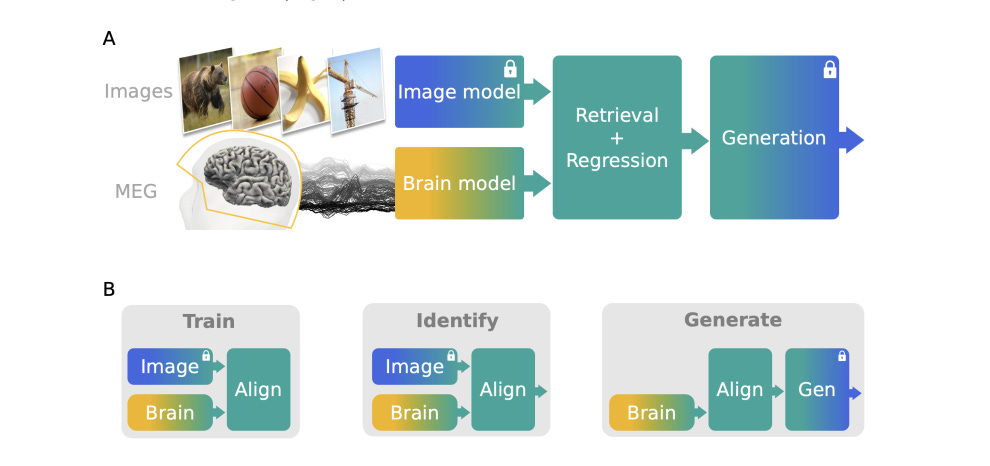
The researchers approached this problem by combining previous work on speech retrieval from MEG (Défossez et al., 2022) and on image generation from fMRI (Takagi and Nishimoto, 2023; Ozcelik and VanRullen, 2023). They have developed a three-module pipeline trained to align MEG activity onto pretrained visual embeddings and generate images from a stream of MEG signals. Their approach is described in the figure below, as provided in the paper/document.
(4) Formulating the Problem Statement(Mathematically)
This section describes the problem formulation for decoding brain activity into images using MEG data. Let’s break it down step by step.
Goal: To reconstruct or retrieve an image that a person is seeing based on MEG brain activity recordings.
(4.1) Key Variables & What They Represent:
For context → We are working with MEG signals recorded while participants were looking at images → one by one.
Here I shall describe how the problem has been formalized/modelled mathematically in the paper:
- \(X_i \in \mathbb{R}^{C \times T}\)
Consider Xi → This is the MEG data recorded when a participant “sees” an image.
i = Index of the image shown to the participant.( 0,1,2,3..)
Let each image be represented by Ii. → I0, I1, I2…
What does the above notation represent? → The recorded data (Xi) falls under/belongs to the set of all real number matrices of the size C x T → where C represents the number of rows of the matrices and T the number of columns. So now we know the format of data received from the MEG technique.
C = Number of MEG channels (sensors) recording brain activity. So, as mentioned earlier, if there are 300 sensors, with each and every one of them recording data, then C = 300 (example).
T = Number of time points in the MEG recording window (how long they record for). Each column in the data Xi is a time point.
- \(z_i \in \mathbb{R}^{F}\)
Now, each image(the original image shown to the participants) → Ii is also converted into a latent representation. What is a latent representation of an image?
The latent representation is like a compressed version of the image with only its essential details. It is extracted using a pretrained neural network (like CLIP or a vision transformer). This means instead of storing pixel-by-pixel data, a compact "meaningful" representation of the image is stored instead.
zi(as shown above) → is a latent representation (compressed vector) of the image Ii.
F = Number of features in the latent representation.
Here, the notation R^F is an F-dimensional real-valued vector space. It’s a singular vector with F number of real values in the vector. For example, if R^4 where F = 4, then zi would look something like
z =[0.21,−0.34,0.98,1.12](random values) as this belongs to the set R^4.
- \(fθ: \mathbb{R}^{C \times T} \to \mathbb{R}^{F} \)\(\hat{z}_i = f_{\theta}(X_i) \)
Now, the researchers define a function named fθ/f theta(as shown above) which maps the MEG signal data gained to the latent representation of an image. This essentially means the model learns to map brain activity to image features.
This is the brain decoding model.
It is trained to take MEG recordings Xi as input and predict z(hat)i, the latent representation of the seen image.
Why? There is no pre-existing formula that directly converts MEG signals into image latent representations. Instead, we train a model (the "brain module" fθ) to learn this function for us and find the best possible transformation. Over time with training, the model adjusts θ\theta(its parameters) to minimize the error in this conversion.
This new decoded latent representation derived from MEG data using the brain module model(z(hat)i) is now compared to the latent representation generated directly from the images(Ii) itself, which is zi. The goal is to make sure z(hat)i is as close as possible to zi, meaning the model correctly learns how to reconstruct the image representation from MEG signals.
(4.2) In Simple Terms:
The participant is shown a sequence of images, and their brain activity is recorded with MEG.
Each image is encoded into a feature representation (zi) using a pretrained image model.
The decoding model fθ is trained to map brain activity (Xi) to image features (zi), meaning it learns to predict what the brain sees.
The better the model, the more accurately it can generate the correct latent representation of the image that can then be compared to the true latent representation of the image to gain the accuracy of the model.
If you are wondering why compare latent representations instead of images directly?
The key reasons are:
Latent representations capture meaning more efficiently
Raw images contain a lot of unnecessary details (background noise, lighting variations, etc.).
A latent representation extracts only the most important semantic information about the image, making it more robust and requiring less computational power compared to raw images.
MEG signals are fundamentally different from images
MEG data is a time-series matrix (C×T), while an image is a grid of pixels (H×W×3).
Directly predicting an image from MEG signals would be extremely difficult due to their very different structures.
Instead, mapping MEG signals to a latent space that already exists for images simplifies the problem.
Pretrained models already define a meaningful latent space
The latent representation zi comes from a pretrained image model (like CLIP).
Instead of training a new model from scratch, we can leverage this already meaningful representation.
This allows the use of existing deep learning knowledge without reinventing the wheel.
So, in short: Comparing latent representations makes the problem computationally easier and ensures that the model focuses on high-level image features rather than pixel-by-pixel accuracy.
(5) Training objectives
As shown in the diagram provided above(Figure 1), the image model, which generates latent representations of the original images, and the generation model, which reconstructs images from latent representations, are both pre-trained and remain fixed throughout the pipeline. The focus of training is therefore on the MEG-to-latent module, which learns the function fθ to map MEG data to image representations. Since this is a self-supervised learning model, it must produce a latent representation z(hat)i that is optimized for both retrieval (identifying the correct image in a self-supervised setup) and generation (ensuring the retrieved latent code is useful for the fixed pre-trained generator). Each of these tasks requires a distinct training objective to ensure the model correctly associates brain activity (MEG data) with meaningful visual representations.
To achieve this, the researchers formulated a combined loss function that balances both image retrieval and image generation, ensuring the model learns an optimal mapping between MEG signals and visual representations.
Note:
Self-supervised learning is a machine learning paradigm where a model learns from data without relying on manually provided labels. Instead, it generates its own supervision signals by defining a learning objective that allows it to infer patterns from the structure of the data itself.
In this study, self-supervision means that the model does not have access to explicit image labels corresponding to the MEG data. Instead, it must learn to retrieve the correct image from a set of candidates by comparing latent representations.
This retrieval task serves as a form of self-supervised signal, guiding the model to learn meaningful associations between brain activity and visual stimuli.
(5.1) Training Brain-Image Mapping with CLIP Loss(Retrieval portion)
The first objective in training the brain module fθ is to identify which image corresponds to a given MEG signal (i.e., brain activity data). This is a self-supervised learning problem because we do not explicitly tell the model which image matches the brain activity—it must learn to figure it out by itself.
To achieve this, the researchers use CLIP Loss, a technique originally developed for learning relationships between images and text but now applied to brain signals and images.
(5.1.1) What is CLIP?
CLIP (Contrastive Language-Image Pretraining) was introduced by OpenAI researchers Radford et al. (2021). Instead of classifying images into predefined categories (like "dog" or "car"), CLIP learns to understand images through natural language descriptions or simply captions.
For example, CLIP doesn’t just learn that an image contains a cat; it learns that the image could be described as:
“A fluffy white cat sitting on a windowsill.”
“A pet looking outside on a rainy day.”
CLIP does this by learning a shared space where the representations of images and their corresponding text captions are close together, while unrelated descriptions are pushed further apart.
(5.1.2) How CLIP Works
CLIP has two separate encoders:
An image encoder (like a Vision Transformer or ResNet) processes images.
A text encoder (like a Transformer) processes text descriptions.
Both encoders project their respective inputs into a shared latent space (think of it like a graph where similar things are clustered together).
The model is trained using a contrastive loss function (InfoNCE loss), which ensures or increases the likelihood that:
The image embedding is close to the embedding of its correct text caption.
The image embedding is far from incorrect captions.
CLIP does not need retraining for new images—it generalizes to unseen objects, making it a powerful zero-shot learning model (requires no labelled training to associate an unknown natural language description to an unknown image).
(5.1.3) Why Use CLIP Loss for Brain-Image Retrieval?
In this research, instead of using text descriptions, we use brain activity (MEG signals) as the second input. The goal is to train a model that learns a shared space between brain signals and images, just like CLIP did for text and images.
However, the full CLIP architecture (i.e., the dual encoders) is not being used here.
Instead, only CLIP Loss is used to train the brain module.
(5.2) Applying CLIP Loss to Brain-Image Mapping
The CLIP loss function used in this research is a variation of InfoNCE loss, first introduced by van den Oord et al. (2018) in their Contrastive Predictive Coding (CPC) paper and later adapted by Radford et al. (2021) for CLIP.
The CLIP loss is applied in both directions(brain-to-image and image-to-brain directions):
Brain-to-Image Direction
Given an MEG recording Xi, the brain module fθ maps it to a predicted latent representation: z(hat)i=fθ(Xi)
This predicted latent representation should be most similar to the latent representation zi of the original image (from DINOv2) and dissimilar to the representations of other images.
Image-to-Brain Direction
Given an original image Ii, we already have its latent representation zi(from DINOv2).
The model ensures that zi is closest to the corresponding z(hat)i=fθ(Xi) (the brain-predicted representation) and not similar to other MEG-derived representations.
(5.2.1) Why Do Both Directions Matter?
Brain-to-Image Matching
Ensures that, given a brain signal, we retrieve the correct latent representation.
Image-to-Brain Matching
Ensures that the latent representation learned by the brain module is truly capturing meaningful features from brain activity, reducing ambiguity.
By matching in both directions, the model is forced to learn a stronger and more precise alignment between brain activity and images.
(5.2.2) Loss formula
(5.2.3) Breaking It Down:
z(hat)i=fθ(Xi) → The latent representation predicted from MEG data.
zi → The actual latent representation of the correct image.
s(⋅,⋅) → Cosine similarity (a measure of how similar two vectors are).
τ(tau, which is the letter that looks like a T) → A learned temperature parameter that scales the similarity scores.( a parameter responsible to decide to what extent can 2 latent representations of images be considered similar → how much emphasis is placed on confident matches)
B → The batch size (number of images considered at a time).
(5.3) Training Brain-Image Mapping with MSE Loss(Generation portion)
The model is not just learning to retrieve the correct image representation—it is also learning to generate an accurate latent representation that closely matches the original image’s latent space. This ensures that the representation can be effectively used as input to a generative model for image reconstruction. To achieve this, the researchers apply a standard Mean Squared Error (MSE) loss on the (unnormalized) latent representations zi and z(hat)i, encouraging the brain-predicted representation to be as close as possible to the true image representation.
(5.3.1) Loss formula
(5.3.2) Breaking It Down:
This loss minimizes the squared difference between the predicted latent vector (z(hat)i) and the actual latent vector (zi).
N → The total number of images in the dataset.
F → The number of features in the latent space.
This ensures that the predicted representation (z(hat)i) is as close as possible to the real one(zi).
The losses serve different training objectives, but the researchers require the model to be trained well in accomplishing both the objectives simultaneously, and therefore, they combine the CLIP loss(retrieval) and the MSE Loss(generation) into a single training objective(a unified loss equation).
This combination is done using a convex combination, which means they take a weighted sum of the two losses, ensuring that the total loss remains balanced between both objectives.
(5.4) Final Loss Equation
(5.4.1) Breaking it down:
L(CLIP): The CLIP-based contrastive loss.
L(MSE): The Mean Squared Error regression-based loss.
λ(lambda): A tunable weight (hyperparameter) that determines the trade-off between retrieval performance and latent space alignment.
If λ is closer to 1, the model prioritizes retrieval (CLIP loss dominates).
If λ is closer to 0, the model prioritizes generation (MSE loss dominates).
A balanced λ ensures that both retrieval and generation are optimized.
(5.5) Why Not Just Use MSE Loss?
One might wonder—since the brain module is just predicting a latent representation z(hat)i, why not simply train it with Mean Squared Error (MSE) Loss?
The problem with MSE loss alone is that:
It does not enforce discrimination between correct and incorrect matches.
The model might collapse to trivial solutions (where all representations become similar).
It does not explicitly teach the model to push apart representations of different images, only to minimize the absolute difference.
CLIP Loss solves these issues by:
Actively pulling the correct representations closer together.
Actively pushing incorrect representations further apart.
This contrastive learning approach leads to more robust representations that generalize better.
Therefore, they use a combination of both CLIP and MSE losses, balancing the advantages of both.
(6) The Brain Module
Now coming to the model being used for the brain module, the researchers are adapting a dilated residual ConvNet architecture from the research of (Défossez et al. (2022)(Paper title → “Decoding speech from non-invasive brain recordings”. → arXiv:2208.12266).
This model is denoted as fθ (i.e., it's the function that transforms MEG data into image representations). Its input(MEG window Xi of shape C×T) and output(latent image representation z(hat)i of shape F) are assigned as described before.
The model is modified according to the needs of the research. The original model from Défossez et al. (2022) produces an output “Y(hat)backbone” (variable name) of shape F′×T meaning:
The temporal structure (time dimension T) is preserved through residual blocks.
Instead of a single latent vector, the original model produces a sequence of T latents.
(6.1) ABOUT THE MODEL
So, what is a Dilated Residual ConvNet?
It’s a type of CNN(Convolutional Neural Network) that is modified by combining 2 key ideas with it:
Residual Connections(From the popular ResNet model) and Dilated Convolutions(also called Atrous convolutions)
This combination allows the network to capture long-range dependencies without significantly increasing computational cost.
Residual Connections(ResNet Concept)
Deep networks such as CNNs suffer from the vanishing gradient problem(gradients propagating become so small or negligible that they do not affect the network in any significant way or have any influence on the output of the model, degrading performance)—as layers get deeper, it becomes harder to train them.
Residual connections solve this by adding a shortcut path that skips layers and lets gradients flow directly. This ensures that even deeper layers still learn meaningful features without degrading performance.
Dilated Convolutions (Expanding the Field of View)
Usually, a CNN applies a small filter(a convolution) of (3 x 3) to the input, but a dilated convolution introduces gaps(dilations) between pixels so the filter covers a larger receptive field without increasing the number of parameters.
It’s like stretching a standard convolutional filter by skipping pixels, allowing the network to "see" a wider region of the input. So if d is the dilation rate(the threshold value to stretch the filter), a 3×3 filter with d=2 covers a 5×5 area while still using only 9 parameters. (It’s like seeing the bigger picture but not having a lot of details about its smaller moving parts)
This is useful in time-series(MEG data) or spatial data because it captures long-range dependencies efficiently.
Why is it useful here?
MEG data is a time-series signal, so the model needs to capture both short-term and long-term dependencies observed through time in the brain signals.
Note:
short-term - fast, immediate, smaller changes/patterns in brain signals
long-term - captures slower, high-level patterns, ex: recognition and memory
Dilated convolutions allow the model to learn patterns over long time windows without increasing parameters(keeping the model size the same).
Residual connections help the model train deeper networks without vanishing gradients.
END OF “ABOUT THE MODEL”
Therefore, by the properties of this model, the temporal structure T is preserved through the residual blocks by making sure the short-term and long-term dependencies are not lost as the model doesn’t process each time-step in the data independently and learns the dependencies between the previous set of time-steps and the next set.
But the described model being used doesn’t output a single latent representation or vector; rather, it preserves the Time dimension(T) and outputs a “sequence” or multiple latent vectors, with each representing the brain activity at time step T.
However, as previously described in the section on the formulation of fθ, the researchers aimed to generate a single latent representation vector for each MEG recording. Specifically, for every image Ii viewed by a participant, the corresponding MEG data, collected over the time-period t, needed to be aggregated into a single latent representation. This output vector was required to belong to the space R^F, meaning it had F features, each represented as a real number.
Therefore, they modified the model according to their needs. They added a temporal aggregation layer to reduce Y(hat)backbone from shape F′×T to a single vector Y(hat)agg (where agg → aggregation) of shape F′.
To do this, they experimented with three types of aggregations:
Global average pooling (averaging over the time dimension).
A learned affine projection (a linear transformation to capture patterns in the time dimension).
An attention layer (learning to focus on the most important time points).
To convert the F′ to the desired dimension of F, after the aggregation, the researchers also add two Multi-Layer Perceptron heads / MLP heads. Each of the heads would optimize for each of the losses (CLIP loss and MSE loss) by learning separately for each loss in Lcombined.
(6.2) What is a Multi-Layer Perceptron?
A Multi-Layer perceptron is just a small fully-connected neural network, which essentially just means that each neuron in every layer(except the output layer) is connected to every neuron in the next layer throughout the network. They are attached to the backbone or the main model to perform specific tasks such as refining the output of the main model for different objectives and more.
(6.3) What role does it play in converting the intermediate output of Y(hat)agg from the shape of F′ to F?
Heads refer to the last part of a model that consists of the output layers. A model can have a singular head for a singular task or multiple heads for multiple tasks, as seen above. Each MLP, therefore, operates on a singular type of loss, which is, in this case, either L(MSE) or L(CLIP). The intermediate output Y(hat)agg, which is the output gained after the temporal aggregation layer, is passed on to both the MLP heads in parallel or simultaneously (in the sense that the intermediate output layer, which is the layer that outputs Y(hat)agg, is connected to both the MLPs, but the MLPs are not connected to one another).
The MLP learn to convert a latent representation of dimension F′ to F to minimize the loss between the predicted latent representation and the original latent representation of the image. Each of them has separate outputs on which losses are calculated according to their respective loss functions, and then the gradients are propagated back through the MLP layers.
After the gradients have propagated through the MLP heads and reached the backbone model, the losses are combined using the L(combined) equation and then backpropagated through the rest of the model, updating the weights of the model to learn a feature representation that benefits both objectives.
(6.4) Optimizing the brain module:
To optimize the brain module, the researchers:
Run a hyperparameter search to find the best:
Pre-processing method for MEG data.
Architecture (number of layers, filters, etc.).
Optimizer settings.
CLIP loss hyperparameters (temperature scaling, batch size, etc.).
The Final Architecture for retrieval contains 6.4M trainable parameters and uses:
Two convolutional blocks (for feature extraction).
An affine projection for temporal aggregation. (a linear transformation followed by a translation(bias shift) that is responsible for converting Y(hat)backbone into Yagg, which is a fixed-size representation that doesn’t contain the time component T)
(6.5) Postprocessing of MSE outputs:
For image generation, the model needs to produce latents that match the statistical properties of the original latents used for training. Since the MSE head predicts latents directly, there can be scale mismatches between the predicted latents and the original latents used to train the generative model.
To correct this, the researchers apply:
Z-score normalization: This ensures that each feature of the predicted latent has zero mean and unit variance.
Inverse Z-score transformation: The predicted latents are re-scaled to have the same distribution as the original latents from the training data.
What this achieves:
Improves compatibility between the predicted latents and the generative model.
Ensures consistency between training and inference latents.
Prevents the generative model from receiving out-of-distribution latents, which could lead to poor image reconstructions.
Why isn’t this done for the CLIP loss head during image retrieval?
For image retrieval, the CLIP loss head doesn’t need to generate latents that match a precise distribution—it only needs to rank images based on similarity correctly.
Retrieval is based on similarity, not reconstruction: CLIP loss ensures that the predicted latent is closest to the correct image latent and farther from incorrect ones. Scaling mismatches don’t affect ranking as long as relative distances are preserved.
Contrastive learning is robust to scale changes: Unlike MSE, CLIP loss is contrastive—it learns relative similarities. Scaling doesn’t significantly impact performance.
Key takeaway:
MSE loss = needs exact reconstruction → requires postprocessing.
CLIP loss = needs similarity ranking → no need for postprocessing.
(7) Image Module, Generation Module, and Optimizations on Latent Space
As mentioned earlier, the researchers do not train the model using raw images. Instead, they use latent representations—high-level feature encodings generated by a pretrained image model. These latent spaces (continuous, high-dimensional spaces where models encode meaningful representations) capture both visual and semantic information.
The brain module is trained to predict these latent representations rather than raw pixel data. The researchers use three types of embeddings:
CLIP-Vision latents – Encodes images using a pretrained CLIP vision transformer.
CLIP-Text latents – Encodes text descriptions from a pretrained CLIP text model, providing semantic information (e.g., object categories).
AutoKL latents – A compressed image representation from a variational autoencoder (VAE), which is commonly used in generative models for reconstructing images.
However, these embeddings are still high-dimensional, which could make training inefficient or lead to overfitting. To simplify the target representations, the researchers select key summary features:
CLIP-Vision → CLS token: A single vector summarizing the entire image.
CLIP-Text → Mean token: The average of all text token embeddings.
AutoKL latents → Channel-average: An aggregated feature map from the autoencoder.
This dimensionality reduction ensures that the brain model learns compact and meaningful representations, making training more efficient while retaining essential information.
The researchers also investigate which types of learned representations align best with brain activity by comparing MEG-derived latents to embeddings from different learning paradigms:
Supervised models (e.g., VGG-19)
Self-supervised contrastive models (e.g., CLIP)
Variational autoencoders (VAE / AutoKL)
Non-deep-learning human-engineered features
By evaluating these different embeddings, they analyse which representations best match MEG activity and which learning paradigm is most biologically relevant. However, while studying this part of the paper, I realised, one open question remains:
Does higher similarity between MEG-derived latents and these embeddings necessarily lead to better image reconstruction?
While stronger alignment may suggest biological relevance, it does not automatically imply that the image generation module will produce more accurate reconstructions. Further investigation into this connection could provide deeper insights into both brain representation learning and generative modelling.
(7.1) Generation Module: From Latents to Images
For image reconstruction, the researchers use a latent diffusion model (similar to Stable Diffusion) conditioned on three inputs:
CLIP-Vision embeddings (257 tokens × 768) – Instead of a single latent vector, this provides a sequence of tokens, capturing different aspects of the image.
CLIP-Text embeddings (77 tokens × 768) – Captures semantic associations from text.
AutoKL latents (4 × 64 × 64) – A compressed representation optimized for diffusion-based image synthesis.
The generation module takes these three embeddings and reconstructs images based on them. To do this, it follows the approach of Ozcelik & VanRullen (2023) (Referenced paper → Natural scene reconstruction from fMRI signals using generative latent diffusion → Another interesting research work!), refining images through:
50 “DDIM” steps – Controls the number of steps in the diffusion process.
Guidance scale – Determines how strictly the model follows the provided embeddings.
Mixing – Likely balances the influence of CLIP and AutoKL latents during generation.
Strength – Influences how much the input image guides the final reconstruction.
By fine-tuning these parameters mentioned above, the researchers optimize the balance between faithfulness to brain-derived latents and realistic image synthesis, enabling reconstructions that reflect both the structure and semantics of the original stimulus.
(8) Time Windows - When should brain activity be captured?
Since MEG data is recorded over time, capturing brain activity in a continuous stream, a key challenge is determining which part of this temporal signal is most relevant for reconstructing images. To address this, the researchers train separate models on different time windows while ensuring that their outputs remain comparable. This allows them to analyse how different phases of brain activity contribute to image generation.
The researchers do this by splitting the data into smaller time windows (e.g., 100 ms, 150 ms, 200 ms → 1500ms). Each time window captures a different phase of how the brain processes a visual stimulus. Early time windows may reflect low-level sensory processing (e.g., detecting edges, shapes) while later time windows may involve higher-level cognitive functions (e.g., recognition, memory recall).
“But Didn’t They Use Temporal Aggregation”? That’s what I thought as well, but the temporal aggregation is for all the changes “within” a singular time window and not for the entirety of the process.
Can they theoretically temporally aggregate all the changes for the complete timeframe? Maybe yes … but that would result in not knowing which time window is the most informative. This also implies that not all time windows contain useful information that is required for image reconstruction. For this problem statement, the researchers require the window in which the brain’s activity best matches deep learning representations and contributes most to accurate image reconstruction.
(9) Training and Computational Considerations
The researchers train cross-participant models on ~63,000 MEG-image pairs using the Adam optimizer (β₁ = 0.9, β₂ = 0.999) with a learning rate of 3 × 10⁻⁴ and a batch size of 128. Early stopping is applied with a patience of 10 (how many epochs the training must continue after the loss starts decreasing) on a validation set of ~15,800 samples, randomly selected from the training set, to prevent overfitting. The final model is evaluated on a held-out test set. Training runs on a single Volta GPU (32GB VRAM)(impressive), and each model is trained three times with different random seeds to ensure stability and reproducibility.
(10) Evaluation of the model
The researchers evaluate the model’s performance using three main types of metrics: retrieval, generation, and real-time/average metrics.
(10.1) Retrieval metrics(Matching MEG Derived Latents to Correct Images):
As you might remember, the model is responsible for selecting the image that is most similar to or most likely the origin of the MEG latent that is now produced by the model. Retrieval metrics are useful because they stay consistent regardless of MEG dimensionality or image embedding dimensionality.
How and Why?
These metrics essentially measure how well the brain-derived representation matches the correct image using → relative rank and top-5 accuracy:
Relative Median Rank → Measures how well the correct image ranks among all candidates, normalized by retrieval set size (independent of dataset size). It normalizes the ranking of the correct image by the retrieval set size, making it independent of feature space dimensions.
Top-5 Accuracy → A standard metric in vision tasks that checks if the correct image is within the top 5 retrieved matches. The method only checks if the correct image is within the top 5 matches, ignoring the actual numerical differences in feature spaces.
Cosine similarity is used to measure similarity between the brain-derived representation and the correct image representation. Since cosine similarity (used for retrieval) compares direction rather than magnitude, it remains stable across different feature spaces.
(10.2) Generation Metrics (Assessing Image Reconstruction Quality)
The evaluation of the pre-trained latent diffusion model (that is responsible for generating images from the produced latents) includes both qualitative and quantitative measures to assess how accurate and realistic the reconstructions are. Since our brains do not reconstruct the picture
Metrics used for comparing reconstructed images with real ones(same metrics used by Ozcelik and VanRullen (2023)):
PixCorr → Pixel-wise correlation between original and generated images.
SSIM (Structural Similarity Index Metric) → Measures perceptual similarity (difference in → contrast, structure, brightness, etc.).
SwAV → Measures similarity using features from SwAV-ResNet50
SwAV (Swapping Assignments between Views) is a self-supervised learning method developed by Facebook AI (FAIR) for learning image representations without labeled data.
SwAV-ResNet50 is simply a ResNet50 model trained using SwAV's self-supervised learning approach, meaning it learns to cluster similar images without explicit labels.
To compare generated images with real images, they extract feature representations(high-level semantic features) from a SwAV-ResNet50 model and calculate similarity.
The researchers also use additional deep-learning-based comparison metrics for high-level feature comparison, such as → realism and semantic accuracy:
AlexNet (2/5 layers) → Checks feature similarity at different layers(2 and 5 of the AlexNet neural network).
Inception pooled last layer → Measures high-level semantic similarity(The final pooled feature vectors from Inception for both images are compared).
CLIP output layer → Evaluates similarity between generated and original images based on CLIP embeddings.
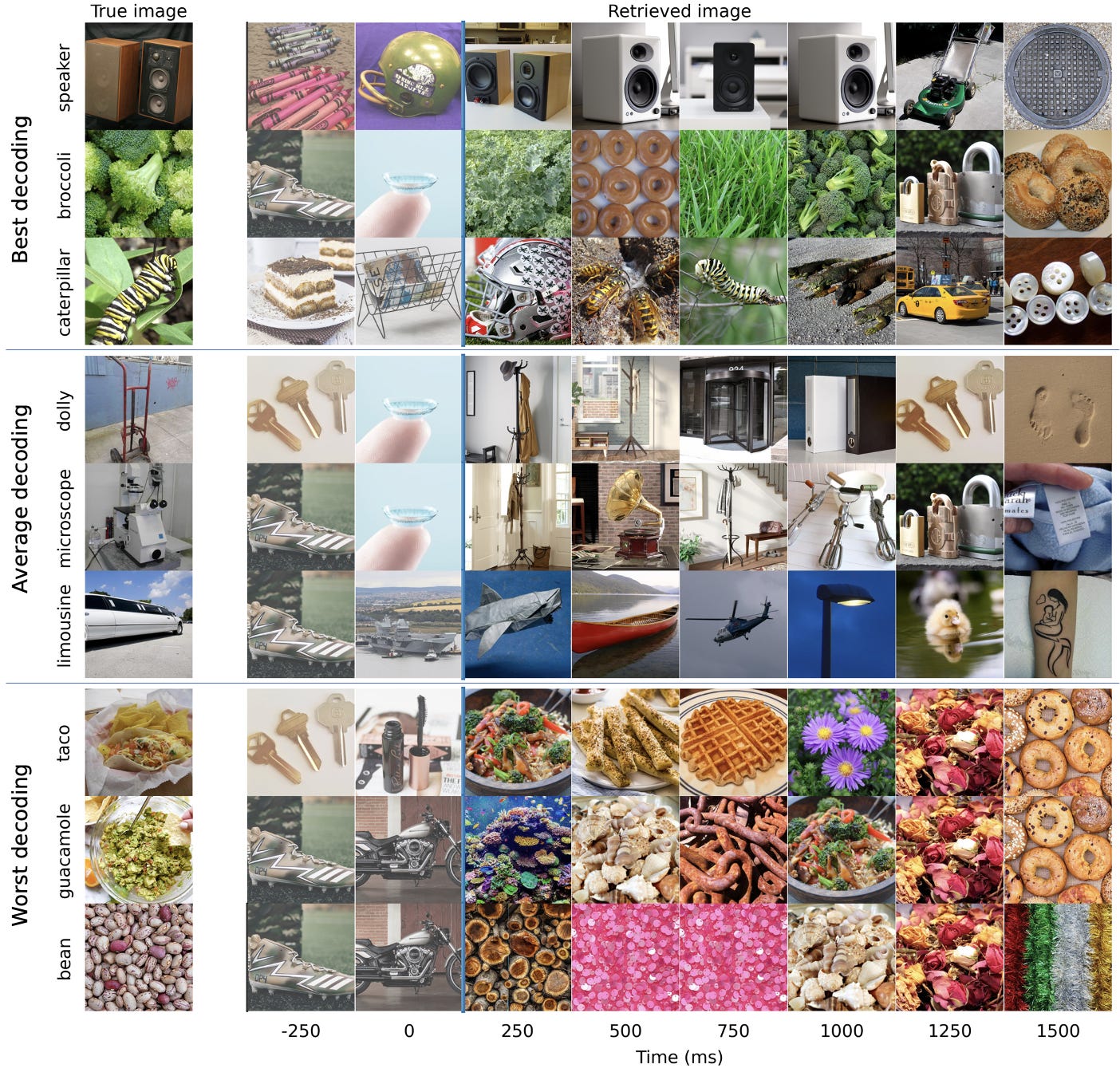
The researchers avoid cherry-picking → To ensure fairness, the test set images are ranked based on a combined SwAV and SSIM score, then split into 15 groups.
From the best, middle, and worst groups, 4 images each are chosen to ensure diverse evaluation rather than only showing the best cases.
(10.3) Real-Time and Averaged Metrics (Handling Multiple Image Presentations)
In fMRI studies, researchers often show participants the same image multiple times and record brain activity each time. Instead of using the raw brain activity from a single trial, they compute an average response across multiple presentations of the same image.
This averaged response is called a "beta value", which helps reduce noise and improve decoding reliability.
The MEG dataset also contains repeated presentations of the same image (i.e., participants see the same image multiple times while MEG data is recorded). Instead of evaluating decoding performance based on a single trial, the researchers average the predicted outputs across all presentations of the same image.
This reduces random variations and makes the decoding performance more stable and accurate. If MEG decoding were evaluated based on single-trial predictions, it might be noisier and inconsistent.
Since fMRI studies use beta values (averaged responses), applying the same averaging method to MEG ensures a fair comparison between MEG-based and fMRI-based decoding.
(11) Datasets Used And Pre-processing Performed
The study utilizes the THINGS-MEG dataset (Hebart et al., 2023), where four participants (2 male, 2 female, mean age 23.25 years) underwent 12 MEG sessions while viewing 22,448 unique images from the THINGS database, covering 1,854 object categories. A subset of 200 images (each from a different category) was repeated multiple times to improve decoding reliability. Each image was displayed for 500 ms, followed by a 1,000 ± 200 ms fixation period. Additionally, 3,659 images never shown to participants were added to the retrieval set to test model robustness.
To process the MEG data, a minimal preprocessing pipeline (Défossez et al., 2022) was applied: (1) Downsampling from 1,200 Hz to 120 Hz, (2) Epoching from -500 ms to +1,000 ms relative to stimulus onset, (3) Baseline correction to remove signal drift, and (4) Robust scaling with outlier clipping at [−20, 20] to stabilize extreme values.
(11.1) Addressing Limitations in the Original Data Split
The original dataset split (Hebart et al., 2023) posed a limitation: the test set contained only 200 images, each belonging to categories already present in the training set. This meant that evaluating retrieval performance only tested the model’s ability to categorize images, rather than (1) generalizing to entirely new categories (zero-shot learning) or (2) distinguishing between multiple images within the same category (fine-grained retrieval).
To address this, the authors introduce two modifications:
Adapted Training Set – Removes images from the training set if their category appears in the test set, eliminating category leakage and enabling zero-shot evaluation.
Large Test Set – Constructed from removed training images, allowing a more rigorous retrieval evaluation that requires differentiating between images of the same category.
(11.2) Comparison with fMRI-Based Models
To benchmark MEG-based decoding, the authors compare their approach against fMRI-based models trained on the NSD dataset (Allen et al., 2022). This is significant because fMRI has historically achieved higher decoding performance due to its superior spatial resolution. By including this comparison, the study assesses whether MEG, despite its lower spatial precision, can still yield competitive decoding results.
This refined dataset design ensures a fair and meaningful evaluation of MEG’s ability to reconstruct images from brain activity while addressing dataset biases and allowing for comparisons with fMRI-based approaches.
(12) The RESULTS
Now we have finally arrived at the results obtained from this research. So, what did the researchers accomplish and how did they accomplish it?
As described earlier in the “Training objectives” section, there are 2 main tasks the model is trained for: (1) retrieval, (2) generation.
(12.1) Retrieval Performance: Which Latent Representations Worked Best For This Task?
The researchers evaluated 16 different image representations (latent spaces) across two models:
A Dilated Residual Convolutional Network (ConvNet) was designed or modified for this study.
A Linear Ridge Regression Model for comparison.
What are linear ridge regression models ?
This model is a variation of the usual linear regression models which is used in the cases where there are a large number of input parameters that might be correlated or in the cases where you want to prevent a linear regression model to overfit on the data.
This is done through a change in the loss formula of a linear regression model. If we take a LRM using the MSE Loss formula, Ridge Regression models add an L2 penalty(sum of the squares of the weights) multiplied to a factor of λ(lambda)
y = target
X= input data
w= weights
λ = regularization strength
(12.1.1) Key Findings
All tested embeddings performed above chance level, confirming that MEG signals contain meaningful visual information.
Supervised models (VGG-19) and multimodal models (CLIP-Vision) showed the highest retrieval accuracy, suggesting they best capture features relevant to brain encoding.
(12.1.2) Performance Comparison: Deep ConvNet vs. Linear Model
The deep ConvNet model outperformed the linear Ridge regression model by 7× or 7 times.
This highlights the advantage of deep learning in decoding brain activity more effectively than traditional methods.
(12.2) Which Representations Were Most Effective?
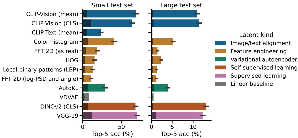
Top-5 retrieval accuracy for the small test set (easier task):
VGG-19 (Supervised learning): 70.33% ± 2.80%
CLIP-Vision (Image-text alignment): 68.66% ± 2.84%
DINOv2 (Self-supervised learning): 68.00% ± 2.86%
When tested on the large test set (harder task):
The best models achieved ~13% accuracy, which is still far above the chance level (0.21%), confirming the model isn't just guessing.
(12.3) Understanding the Two Test Sets
Small Test set → 200 images, Task Difficulty: Category-level recognition, ~70% (Top-5), 2.5%
Large Test set → 2,400 images, Task Difficulty: Fine-grained image retrieval, ~13% (Top-5), 0.21%
The small test set required recognizing category-level features (e.g., "dog").
The large test set required distinguishing fine-grained details between similar-looking images (e.g., different breeds of dogs).
(12.4) Why Do Some Representations Work Better?
Top Performers(latents):
VGG-19 (Supervised Learning) → Well-trained on object categories.
CLIP-Vision (Image-Text Alignment) → Captures high-level semantics.
DINOv2 (Self-Supervised Learning) → Learns structure from large-scale unlabelled data.
Poor Performers:
Feature-engineered representations (e.g., colour histograms, HOG, LBP) performed poorly.
These only capture low-level image statistics, whereas deep networks capture higher-level semantic meaning.
(12.5) Deep Learning vs. Linear Models: A Clear Winner
Deep ConvNet significantly outperforms the linear decoder.
This suggests deep models can learn richer, more abstract patterns from MEG data.
The performance gap between the small and large test sets reflects the increasing difficulty of fine-grained retrieval.
(12.6) Final Takeaways
Deep learning significantly improves decoding performance over traditional linear models.
Supervised and multimodal representations (VGG, CLIP) align best with human visual processing.
MEG signals contain structured, decodable visual information, supporting future brain-to-image translation research.
Predictions of image latents were done in 2 ways, The first setup had a singular full-time window input of MEG data(500- 1000ms after stimulus onset → when 500 to 1000ms after the test subject looked at the image), which gives out one prediction per image representation. This answers the question: “How well can we decode image identity when we give the model the entire window of brain activity?”
In the second setup, whose results can be seen in Figure X, the analysis was repeated on 100ms sliding windows (i.e., each input to the model spans 100ms of brain activity) with a stride of 25ms (producing inputs from 0–100ms, 25–125ms, 50–150ms, and so on). Because the windows overlap heavily, this yields a continuous series of retrieval outputs approximately every 25ms, rather than just four discrete outputs per 100ms. For visual clarity in the graph below, they focus on a subset of the various image latents used in the first setup. (I’m not entirely sure if they did this for both the models(linear ridge and the convnet, I am assuming further details would be mentioned in the appendix of the paper, or I have missed something and these results are for the convnet)
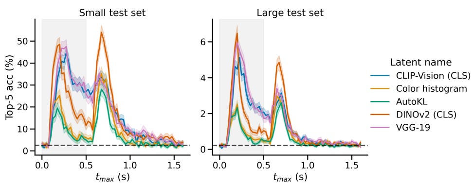
From the graphs for both datasets, the following observations can be made.
(1) As you can see, there are 2 very clear peaks in each graph. The authors observed the first peak at about 200-275 ms after image onset and the second one for windows ending around 150-200 ms after image offset.
First peak → Possibly the brain forms a strong initial representation while seeing the image.
Second peak → Brain still processes the image even after it's gone (post-perception processing, maybe memory-related).
Further analysis shows that the 2 peak intervals contain complementary information(not redundant) for the retrieval task, after which performance goes back to chance level. Meaning the brain is encoding different but useful information during the first and second peaks.
The first peak mostly reflects direct visual perception (the brain seeing the image).
The second peak likely reflects memory consolidation, abstract processing, or mental reactivation of the image.
If you combine information from both peaks (early and late brain signals), retrieval performance gets better than if you use either peak alone.
Each peak adds something that the other doesn't fully capture.
We can infer that retrieval gets stronger if the model can use information in the time periods where the peaks occur.
(2) The other observation made is that the self-supervised DINOv2 model latents yield the highest peaks in performance as seen in the graph, which is especially significant in the second peak, which happens after image offset.
The authors further state that:
1. Retrieved images are mostly from the correct category (e.g., “speaker” or “broccoli”), → meaning the brain decoding model can guess the right kind of thing the person saw.
2. This happens mostly during the early time window (t ≤ 1 second),
→ meaning the brain’s representation is strongest and most decodable soon after seeing the image.
3. The retrieved images don't share obvious or intuitively recognizable low-level features (like colors, shapes, textures) → meaning the model isn’t just picking up simple visual details — it’s more about high-level, semantic recognition (e.g., “this is a food” or “this is a machine”), not pixel patterns.
This reconfirms that the brain responses tied to both onset and offset (image appearance and disappearance) contribute to decoding.
And it can be inferred that category-level information (i.e., “this is a broccoli”) emerges as early as 250 ms after the image appears. And this is seen from the resulting images derived by brain decoding, provided by the authors.
We can interpret the following from the above
Visual understanding in the brain is fast: Around 250 ms, your brain already categorizes what you’re seeing.
High-level concepts dominate early: The brain isn't just processing raw shapes — it's forming meaningful labels ("food", "object") extremely early.
Image offset (disappearance) still matters: After the image is gone, the brain continues refining or "closing off" the visual memory, and this lingering trace can still be decoded.
Decoding isn't based on pixel-level similarity: The model isn’t cheating by matching low-level image properties. It’s learning what the brain "thinks" the image is.
This can be better understood from the visualization provided by the authors below
(12.7) Now, Coming Back to Generation
In addition to retrieval tasks, the authors aimed to tackle a more challenging and practical goal: generating images directly from brain recordings.
While retrieval offers promising decoding performance, it inherently assumes that the true image is already present among a set of candidates — an unrealistic constraint for real-world applications where the objective is to reconstruct novel images purely from brain activity.
To move beyond this limitation, the authors took the following approach:
They trained three distinct "brain modules" to predict visual feature embeddings from MEG data, enabling image generation conditioned directly on neural signals. (More details about these brain modules are discussed in the earlier section of this blog under "Generation Module.")
Building on their retrieval framework, they tested two strategies for conditioning image generation:
Growing Windows:
Gradually increasing the amount of MEG data from [0, 100] ms up to [0, 1500] ms after stimulus onset, to observe how generation improves as more temporal information is made available.Full Windows:
Using a wide window spanning from -500 ms before onset to +1000 ms after onset, capturing a broader sweep of brain dynamics.
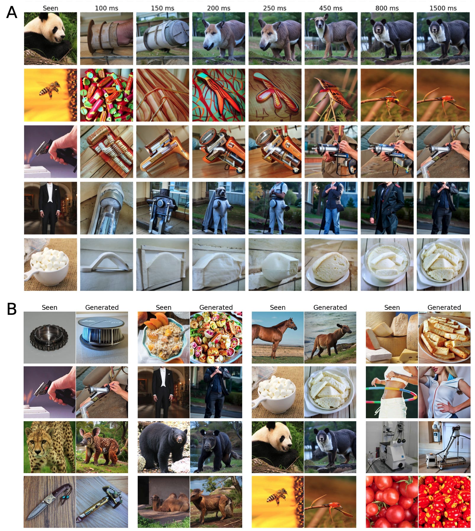
Their results, showcased in Figure 4 and Appendix H, reveal that while generated images often preserve the high-level category of the original stimulus (e.g., "vegetable" or "speaker"), they tend to lose low-level visual details like precise position, color, and texture.
A deeper sliding window analysis further showed that:
Early brain responses (soon after onset and around offset) are primarily associated with low-level sensory features.
Brain activity between 200–500 ms after onset appears to encode higher-level semantic information, critical for categorizing what the image represents.
These findings suggest that as visual information unfolds in the brain, early stages prioritize fine-grained sensory details, while later stages rapidly abstract these into categorical, conceptual representations — an important insight for future brain-to-image generation systems.
(12.8) Why Are Low-Level Details Missing? Comparing MEG and fMRI Reconstructions
One important question the authors address is: Why do the images generated from MEG recordings tend to lose low-level visual details (like texture, color, or object position)?
To investigate whether this limitation comes from the brain-to-image pipeline itself or from the nature of MEG signals, they ran a key comparison:
They applied a very similar generation pipeline — using simple Ridge regression (a standard linear model) — on an analogous fMRI dataset (Allen et al., 2022; Ozcelik and VanRullen, 2023).
Notably, the fMRI-based reconstructions successfully preserved both high-level and low-level features of the original images (see their Figure S2).
This comparison led to an important conclusion:
→ It is not the decoding method that struggles to reconstruct low-level features, but rather the MEG signals themselves that are harder to decode in this respect.
In other words, MEG, due to its nature — offering high temporal resolution but relatively low spatial resolution — may capture the broad timing of neural events very precisely, but may lack the fine-grained spatial information necessary for detailed visual reconstruction.
fMRI, on the other hand, offers high spatial precision (at the cost of temporal delay), making it better suited to capture the detailed structure of visual scenes.
Thus, the inability to generate highly detailed images from MEG is not a flaw in the model, but a reflection of the different kinds of information that MEG and fMRI can access about brain activity.
(13) Wrap Up - There was a lot to cover, but we are finally done, mostly…
(13.1) Related Works
So, has there been no previous research or any form of work that accomplished a similar objective? According to the authors, as of their time of research, there was, to their knowledge, no MEG decoding study that learns end-to-end to reliably generate an open set of images.
This research builds on past studies that have sought to understand how the brain processes visual information by analyzing brain activity.
Previous work has used linear models to either classify a limited set of images based on brain activity or predict brain activity from images’ latent representations (Cichy et al., 2017).
Representational Similarity Analysis (RSA) has also been used to compare how images and brain activity relate to each other (Cichy et al., 2017; Grootswagers et al., 2019).
These studies mainly focus on classifying a small number of image categories or comparing pairs of images, often using simpler models like linear decoders.
In contrast, the current research shifts away from focusing solely on classification. It seeks to decode brain activity in a way that generates a broader set of images, rather than just identifying specific categories. This approach is more complex and involves deep learning techniques to handle the richness of brain activity.
(13.2) Impact
This study makes significant methodological contributions both for basic neuroscience and practical applications. Generating images from brain activity could give researchers a clearer view into how the brain processes different aspects of a visual scene. This method makes it easier to pinpoint what kinds of features (e.g., object parts, textures) are represented in the brain at different stages of visual processing. Previous work on decoding subjective experiences, like visual illusions (Cheng et al., 2023), has shown how generative decoding could uncover the brain's mechanisms of subjective perception.
On the practical side, the ability to generate images from brain signals has several applications. For example, this method could be used to help people with communication challenges, such as those with brain lesions, through brain-computer interfaces (BCIs). However, current methods still rely on neuroimaging techniques like fMRI, which have lower temporal resolution compared to methods like MEG or EEG. This suggests that future work could extend this to EEG, which is widely used in clinical settings due to its high temporal resolution.
(13.3) Limitations
Despite the promising results, the study acknowledges a few limitations in the decoding process. One challenge is that MEG (Magnetoencephalography) has lower spatial resolution than fMRI (7T fMRI), which makes it less effective at capturing fine details of visual processing. Additionally, the method used relies heavily on pre-trained models, which may not always generate the best results. While these pretrained embeddings (image features) perform better than older methods like color histograms or HOG (Histogram of Oriented Gradients), there’s still room to improve by fine-tuning the image generation models or integrating different visual features.
(13.4) Ethical Implications
The rapid development of brain decoding technologies raises important ethical concerns. For instance, as these methods get better at decoding perceptual experiences, they could infringe on mental privacy. It's crucial to consider consent, especially since the decoding accuracy is much higher when subjects are focused on perceptual tasks, but much lower when they're imagining things or engaged in disruptive tasks. These findings suggest that while decoding can be highly informative, it must be approached carefully to ensure that individual privacy is respected. Open and peer-reviewed research practices are encouraged to address these issues transparently.
(13.5) Conclusion
In summary, the study advances the ability to decode visual processing in the human brain, moving beyond simple classification to generate images based on brain activity. While there are still challenges, particularly with improving spatial resolution and fine-tuning models, this approach could lead to significant breakthroughs in both basic neuroscience and practical applications, such as brain-computer interfaces for communication. However, ethical considerations, especially around privacy, must remain a priority as these technologies develop.
(14) Sources:
(1) Find the paper here: Link to paper
(2) Link to the author’s blog post on the paper(acts as a short summary): Link to Blogpost
(3) AI - ChatGPT for writing assistance and understanding the material, DALL-E 3 for image generation